Product Range Consistency: The Key to Long-Term Success in Online Retail

In the world of e-commerce, where competition is growing literally every day, product range consistency is becoming not a luxury but a vital necessity for business survival. Imagine: your online store offers thousands of products, but after a couple of months, half of them are outdated, don't sell, or are no longer relevant. This is a direct path to customer loss and a drop in conversion rates. A stable assortment doesn't just mean variety; it's a skillful balance between seasonal hits, perennial bestsellers, and innovative new products. This balance ensures your online store's stable income, minimizes risks, and flexibly adapts to market changes.

Why is this so important? According to research by Statista, 70% of shoppers switch to competitors due to an outdated or limited assortment. However, a sustainable approach can increase sales by 20-30%. This figure has already been proven in practice. It's essential to properly understand the issue of assortment stability, understand how to correctly calculate the necessary indicators, and implement them in practice.

This is precisely the topic of today's review. In particular, we will now discuss why assortment stability is a crucial aspect of stable sales. We will focus on calculating the corresponding coefficient for different product categories. Let's consider additional factors that directly impact assortment stability. The information provided will help you create a product assortment for your catalog that will ensure regular sales and profits, and, along with it, increased loyalty from your target audience.

Assortment Stability: The Foundation of a Stable E-Commerce Business

Assortment stability is a key metric that evaluates how effectively a company can maintain a stable and predictable selection of products for sale. This indicator tracks the dynamics of changes in the number of items in the assortment over a selected period, be it a month, quarter, or year, helping to identify trends of growth, stagnation, or decline. In the online retail niche, where customers expect instant access to the products they need, stability is especially important. This is what prevents "empty shelves" on virtual storefronts and ensures a positive user experience, minimizing the churn of potential customers due to the lack of expected products.

This stability, in practice, brings tangible benefits not only to retailers and marketplaces like Wildberries or Ozon, but also to manufacturers seeking long-term, unreliable partnerships. Judge for yourself:

1. Significantly accelerates customer service. Shoppers spend less time searching because they know the selection is consistent and can quickly find the right product, whether it's a favorite smartphone model or seasonal clothing.
2. Customer loyalty is enhanced. Consistent availability of key items creates a sense of reliability, encouraging customers to return and recommend the store to friends, which directly impacts repeat purchases and reviews.
3. Sustainability enables the standardization of business processes, from procurement and warehouse storage to product display and delivery logistics. This simplifies supply chain management in a dynamic online marketplace.
4. Cost minimization. This is due to reduced labor costs for revaluation, inventory control, and marketing of new products. Savings in analysis time and money spent on excess inventory that could sit unsold in warehouses are observed.

At its core, the assortment stability ratio is a quantitative metric calculated as the ratio of stable products to the total number of SKUs (usually using the formula:

K = (Number of stable SKUs / Total number of SKUs) x 100%).

The higher this ratio, which ideally should be at least 70%-80%, the more stable the assortment, indicating business maturity. In practice, it has found application in strategic management, particularly during the adjustment of assortment policy, including the removal of "dead" products, inventory optimization to avoid shortages or overstocks, and the organization of uninterrupted supply to retail outlets, distributors, or online platforms. Ultimately, focusing on sustainability helps not only survive seasonal fluctuations and competition but also scale sales, turning your product range into a powerful growth tool.

How to Calculate the Assortment Sustainability Ratio

The Assortment Sustainability Ratio is an important metric that evaluates the dynamics of changes in the breadth and depth of a product offering over time. Essentially, it shows how stable the number of products on sale will be over a given period, ranging from a month to a year. This helps anticipate the risk of empty shelves or avoid an oversupply of outdated items. In online retail, where customers expect constant access to product range across multiple platforms, this metric is especially valuable. The point is that it reflects a business's ability to adapt to seasonal fluctuations in demand without losing customer loyalty and minimizing losses from unsold inventory.

Currently, there are several methods for calculating the stability ratio, and the choice depends on the specifics of the company, available data, and established analytical practices. One basic approach involves comparing the number of stable SKUs, or stock keeping units, at the beginning and end of the reporting period. An analyst can use a simple formula:

Ku = (Quantity of stable products at the end of the period / Total quantity at the beginning of the period) × 100%

However, for greater accuracy, more complex models that take into account turnover and seasonality are used. The main thing is to collect up-to-date inventory data from your business's accounting systems, whether ERP, CRM, or marketplace analytics. This will ensure the most objective and relevant calculation.

The calculation can be performed at the enterprise level, providing an overall picture of the product range, or for individual product groups, such as electronics, clothing, or food. This allows for focusing on problematic segments. It is especially recommended to calculate the coefficient separately for products with different turnover rates. For example, a batch of fresh baked goods or fruit can sell out in 2-3 days, while household appliances or furniture may sit in the warehouse for months. Comparing such categories is inappropriate, as it distorts overall stability.

Similarly, seasonal items should be excluded from calculations, as winter jackets in the summer or Christmas decorations in April will clearly not be in demand and are often temporarily unavailable. However, they will also be stored in the warehouse until the start of the new season. Therefore, their absence could lead to the calculated stability coefficient being incorrect and ultimately leading to incorrect management decisions.

The stability coefficient value ranges from 0, indicating complete instability (i.e., when the product range changes dramatically), to 1, indicating perfect stability without fluctuations. The closer your calculated indicator is to 1, the more stable the product range, indicating effective inventory management and demand forecasting. In academic literature on merchandising, as well as on specialized online platforms, current benchmarks for various business formats are presented:

In small convenience stores focused on everyday goods, the ratio can reach 0.90. This is entirely reasonable, as the constant availability of basic items like bread, milk, and household chemicals is essential.

In an online context, these standards help optimize product cards and recommendations, increasing conversion. Regularly monitoring the ratio allows you to adjust purchasing in real time and avoid overproduction.

• For supermarkets and department stores, the ratio is 0.80. This allows for a balanced selection of products with seasonal new items.
• For specialty stores (such as electronics or clothing), the ratio is 0.75. Here, a focus on narrow product categories is taken into account.

Now let's take a closer look at the various options for calculating the stability coefficient.

Basic Formula for the Stability Coefficient

The assortment stability coefficient serves as a reliable indicator of the stability of a product supply, showing how consistently a certain list of items is available for sale over a given time period, ranging from a few hours to a week. This is especially relevant in online retail, where customers expect products to be available 24/7, and fluctuations can lead to lost sales. Regular inventory checks are conducted to determine the actual number of available varieties.

Their frequency depends on the inventory turnover. Thus, for fast-selling, or most popular, items, such as clothing or accessories, daily monitoring is optimal, while for more durable items, such as furniture or appliances, this period would be weekly. These audits capture the actual state of the product range, helping to identify bottlenecks in logistics or procurement.

The basic calculation of the stability coefficient is performed using a standard formula that takes into account actual data from several audits:

Ku = (RF1 + RF2 + ⋯ + RFn) / Rp x n

Here:

• RF is the number of varieties, i.e., models or SKUs, actually available for sale at the time of each audit;
• Rp is the planned number of varieties according to the assortment plan for a given product group;
• n is the total number of audits performed.

This approach allows for a quantitative assessment of stability, where a value closer to 1 indicates high product range reliability, while a low value indicates the need for adjustments. In e-commerce, such calculations are integrated into analytical tools, including Google Analytics or internal marketplace dashboards, to respond as quickly as possible to changes in demand.

To better understand how this works in practice, let's look at an example from an online clothing store. Marketers conducted four checks throughout the day to assess the stability of key product categories they offered: T-shirts, jeans, and dresses. The plan assumed the marketplace had 10 T-shirt styles, 8 jeans, and 10 dresses in its assortment. The results can be found in the table below, which summarizes the actual quantities for each category.

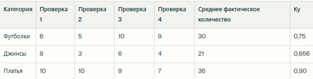
The calculation procedure for each category is as follows:

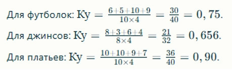
From this data, it is clear that the product range in the "T-shirts" and "jeans" categories exhibits instability throughout the day, as the resulting coefficient is below 0.8. This means there are frequent gaps in inventory, possibly due to delays in inventory updates or peak sales. This can discourage customers who can't find the styles they want when they need them and instead switch to competitors. In the case of dresses, stability is higher, indicating effective planning. However, to improve performance, it is recommended to strengthen supply monitoring and automate low-inventory notifications so that the overall QU in the store approaches the target value of 0.80-0.90. This can increase loyalty and sales.

Calculation using the coefficient of variation

If you read specialized academic literature on merchandising and marketing, you'll notice how often an alternative method for assessing assortment stability—the coefficient of variation—is mentioned. It is claimed to allow for a more in-depth analysis of the variation in product availability data. This approach is somewhat more complex than the basic formula discussed above, as it takes into account statistical variability. However, it provides more accurate results, accounting for even the smallest nuances.

This will be especially relevant in dynamic online retail sectors, where inventory fluctuations can be caused by peak warehouse loads or seasonal demand. This metric helps not only identify product instability but also understand its causes. For example, this could be due to logistical delays or uneven imports. This parameter will be critical for many marketplaces, as product outages lead to immediate customer churn.

The formula for calculating the stability coefficient in this case is as follows:

Ku=1−V

Here:

• V is the variation coefficient, expressing the relative variability of the indicator. This method indicates that the smaller the variation in product availability, the greater the stability of the assortment, and that its coefficient approaches 1. This coefficient of variation is a fundamental statistical measure that assesses the degree of dispersion of values around their mean, normalizing data for comparison across categories. It is calculated as the ratio of the standard deviation (σ) to the arithmetic mean:

V=σ/х

Often in decimal form or as a percentage. The calculation involves several steps: first, the mean value is found across tests, then the deviations from it, the squares of these deviations, their average value, and the root mean of the σ. The calculation process is extremely extensive and requires precision to avoid misinterpretations. Therefore, for practical tasks, specialized online calculators are often used, which are built into specialized platforms or solutions like Excel, which include the AVERAGE() and STDEV.V() functions. This significantly simplifies automation for large e-commerce datasets.

Let's consider another example based on the same products and data we used in the calculations in the previous step. So, we have an online clothing store and the results of four availability checks for models in the categories T-shirts (6, 5, 10, 9), jeans (8, 3, 6, 4), and dresses (10, 10, 9, 7). These values are entered into the coefficient of variation calculator to calculate V, and then Ku.

The results are presented in the table below, demonstrating the impact variation has on the overall stability indicator.

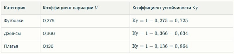
In this scenario, the coefficient of variation for T-shirts (0.275) indicates moderate variability, possibly caused by the rapid sale of popular sizes. This ultimately reduces the stability indicator to 0.725. While this indicator is generally acceptable, it still requires monitoring.

For jeans, we obtain V = 0.366, which in itself indicates high instability, largely due to seasonal fluctuations. The resulting KU is 0.634, which is too low for a comfortable shopping experience and may indicate conditions where customers are at risk of not finding the product they need.

Dresses exhibit minimal variation (0.136), providing high stability (0.864), which is ideal for basic items.

Such calculations help retailers adjust purchasing as quickly as possible by integrating data from CRM systems, while improving the overall effectiveness of their product range, even in highly competitive environments.

Stability Coefficient for Individual Products

Assortment stability analysis can be further refined by assessing the length of time a specific product has been available for sale. This solution is extremely useful in cases where the most accurate and detailed monitoring is needed for individual items, rather than for general product groups. This approach is ideal for small businesses or niche online stores where the product range is limited to dozens of SKUs. In such conditions, it is important to track why a particular product frequently "disappears" from the storefront, as this has a direct impact on user reviews and conversion rates. In e-commerce, this helps identify supply issues or seasonal demand, as well as quickly adjust product availability and avoid penalties for incomplete product range, which is especially relevant for various marketplaces.

In this case, the stability coefficient is calculated using a simple proportional formula that reflects the percentage of time available:

Ku = t / T;

Here:

• t — the number of days the product was on sale. That is, this is the actual number of days or hours the product was on sale and available for order.
• T — The number of days in the analyzed period (month, quarter, year). This is the overall analysis period, i.e., 30 days per month, 90 days per quarter, or 365 days per year.

Two main methods are used to determine t: manual daily inventory monitoring through on-site inspections at offline locations or screen shots of inventory cards in online systems, or automated data analysis from inventory management software, such as ERP, 1C, or marketplace analytics, where balances and statuses are recorded. The second option is preferable for large-scale projects, as it minimizes errors and allows integration with sales reports, increasing accuracy to 95-99%.

We would like to draw your attention to the fact that in this case, the coefficient is calculated individually for each product. Therefore, to evaluate the entire group or the entire assortment, it is necessary to sum the t values for all items and divide them by the sum of the planned T multiplied by the number of products. This yields an aggregate QI, useful for strategic planning. If it's below 0.8, it's worth reconsidering logistics or suppliers.

Here, we'll also look at an example, but this time, we'll focus on an online household chemicals store. In October (30 days), we analyzed three popular products: liquid soap, laundry detergent, and disinfectant spray. Liquid soap was out of stock for two days due to a delivery delay (t=28), laundry detergent was in stock for the entire month (t=30), and disinfectant spray was in stock for 25 days (due to peak demand). The calculation results are presented in the table below.

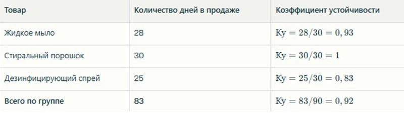
Here, the Ku for liquid soap (0.93) indicates high stability, suitable for a basic product, while the disinfectant spray (0.83) signals the need to build up a buffer stock during periods of increased seasonal illnesses. The overall coefficient for the group (0.92) is an excellent result, close to ideal for everyday products. In this way, we can use calculations to confirm management effectiveness, which will foster customer loyalty, as customers will always be confident that they won't always be able to find the product they need at their favorite store.

Share of Products in Steady Demand

Assortment stability can also be analyzed through the prism of the share of products that demonstrate consistent and predictable demand. Here, we're talking about an alternative approach that focuses on "evergreen" items, those that ensure stable turnover regardless of external fluctuations. This approach is especially useful in online retail, where seasonal trends change quickly and core products form the foundation of customer loyalty. It helps identify "anchor" products. Products for each marketplace, minimizing the risk of impulse hits whose demand quickly declines, and optimizing marketing efforts by focusing on proven bestsellers.

Demand for a company's products is influenced by many factors, from pricing policy and consumer expectations to seasonal trends, economic conditions, and even weather conditions. However, there are categories with high, stable demand. These are products that customers purchase regularly over months or years without any sudden sales declines. These include essentials such as milk, meat, fish, eggs, toilet paper, shampoo, toothpaste, or even basic tools like screwdrivers. Interestingly, demand for food products is usually more stable, as they represent genuine daily needs, than for non-food products, where the influence of fashion or innovation is stronger. This is confirmed by e-commerce analytics data, where product categories such as FMCG show a demand variation of only 10-15% from year to year.

To calculate the stability coefficient in this context, a proportional formula is used that reflects the share of "stable" items in the total assortment:

Ku = Y / Shd

Here:

• Y is the number of individual products or product groups enjoying stable demand. They are determined directly by sales over a certain period of time, for example, if a model is sold monthly without interruption;
• Shd is Actual product range breadth, i.e., the actual total number of products or product groups at the time of analysis.

This method is easy to implement. Data is taken from sales reports, whether from a CRM system or marketplace analytics, where items with a constant turnover are identified. Incidentally, it should be at least 80% of the planned turnover. A high Q, i.e., close to 1, indicates a focus on reliable products, which ultimately reduces the costs of storing and advertising "dead" inventory.

Let's consider an example from a specialized online smartphone store offering 24 models of various brands and specifications. Marketers analyzed quarterly sales data and found that only 12 models enjoyed stable demand, characterized by consistent purchases and no seasonal dips. These are mostly basic, mid-range options with popular screens and cameras. The calculation looks like this:

Ku = 12/24 = 0.50

According to expert recommendations, the optimal K value for a specialty store is 0.75. This balance between variety and stability ensures 70-80% of revenue comes from anchor products. This result is significantly below the norm, indicating an overabundance of niche or outdated models. This means it's worth reviewing the product mix and removing or replacing 8 unpopular models with updated, high-potential alternatives. As a result, the stability coefficient will increase, allowing the business to offer truly in-demand smartphone models, which is guaranteed to increase conversion and minimize the risk of warehouse downtime.

Factors Affecting Assortment Stability

Assortment stability in online retail depends on a variety of external and internal factors that determine how consistently products are available to customers across various marketplaces. These factors can cause fluctuations in availability, impacting conversion and loyalty. According to current analytical data, an unstable product assortment leads to 15-20% lost sales due to "empty" cards. Understanding key factors helps retailers anticipate risks, optimize purchasing, and maintain an optimal balance between product diversity and reliability, especially in the context of rapid e-commerce growth, which is relevant in the second half of 2025.

So, here we discuss the following key factors:

1. Demand fluctuations. Product demand is confirmed by significant variations depending on the time of day, day of the week, month, or season. This is precisely what directly impacts product assortment stability. For example, in an online clothing store, users are more likely to search for everyday items like work T-shirts in the morning, and dresses for special occasions in the evening. This means that recommendations need to be updated fairly quickly. Analyzing demand through tools like Google Analytics or built-in marketplace analytics allows you to anticipate these shifts, taking into account seasonality, whether it's peak demand for jackets in the fall or flip-flops in the summer, as well as competitors' actions, including flash sales on Ozon, which can literally "steal" traffic.
2. Supply Stability. Regular product receipts are the foundation of sustainability, as interruptions in the supply chain can lead to product shortages both in warehouses and at retail outlets. This is especially critical in e-commerce: delays from logistics partners can easily paralyze sales. Furthermore, manufacturers seek uninterrupted supplies of raw materials, packaging, and components for continuous production. For example, if an electronics supplier is a week late with a batch of smartphones, product cards become empty, causing customer attrition. The solution to this problem is Supplier diversification and SLA (service level agreement) contracts to minimize risks.
3. Inventory size. Warehouse availability and inventory volume determine how much a company can buffer demand fluctuations. However, a balance is key: excess product leads to "frozen" assets, while shortages lead to lost sales. Not all retailers have large logistics hubs, so it's important to optimize inventory using ABC analysis (A = high-liquidity products, C = low-liquidity products) to avoid problems like expired cosmetics or obsolescence of gadgets. In an online format, where delivery is expected within 1-3 days, it's necessary to maintain an optimal inventory for approximately 7-14 days of sales. This will ensure a stable 95% product availability and also reduce storage costs by up to 20%.
4. The need to update the product range. Retailers and manufacturers are constantly striving to expand their share of products with stable demand. However, it's important to understand that consumer preferences evolve in response to trends. This means a highly flexible approach to product assortment is essential. For example, in the home appliance category, yesterday's hit mop-vacuum cleaners are giving way to more advanced smart devices, such as robot vacuum cleaners. Without constant product rotation, your product assortment loses its relevance. To avoid risk, we recommend regularly conducting audits using specialized SEO tools, such as Ahrefs and Serpstat, to promptly identify outdated SKUs and introduce new items. This will allow you to strike a delicate balance between stability and innovation, ensuring your sustainability coefficient remains at least 0.8.

Summing Up

Assortment stability is, without a doubt, the foundation of a stable online retail business. A proper product balance minimizes risks, enhances customer loyalty, and increases conversion by 20-30%. In today's article, we carefully examined the stability coefficient, discussed how to correctly calculate it based on certain input parameters, and examined influencing factors. We also want to point out that regular analysis through a product matrix allows you to optimize inventory, adapt to current trends, and avoid "empty shelves" both on marketplaces and in traditional online stores.

The last point we'd like to draw your attention to is the need for regular competitor monitoring. Mobile proxies from MobileProxy.Space will help you complete your upcoming work as efficiently as possible and ensure stable parsing of demand and price data. This service provides anonymous and secure access to websites, IP-address rotation, geolocation to bypass regional blocking, and accurate analytics without the risk of being banned or otherwise restricted.

You can learn more about these mobile proxies here. We'd like to point out that you can test this product completely free for two hours, ensuring its high efficiency and ease of use. Also, please note our current pricing plans and the option that best suits your needs, with durations ranging from 1 day to 1 year. If you have any further questions, please visit our FAQ section or contact our technical support team, available 24/7.

Comparte el artículo: